Vehicle Depreciation Predictor

Overview

Buying a car is one of the largest expenses most people make, and one of the fastest-depreciating. Dealers and large fleet operators price vehicles with proprietary data and models; private buyers get calculators that apply a fixed curve to the purchase price and the vehicle’s age.

This project is an end-to-end platform that predicts a vehicle’s value year by year for the next six years, and explains which characteristics of that specific vehicle push the value up or down. It covers the full path from raw data to a deployed product: a data pipeline and model selection following CRISP-DM, an explainability layer, a containerised prediction API, and a web interface.

The model is trained on U.S. market data. European datasets of comparable size were not openly available, and scraping European listing portals would have conflicted with their terms of use, so the project uses an open dataset instead.

Architecture

The production system is decoupled into a frontend and a prediction service, so the interface stays fast and independent of model load.

1. 01Web interfaceNext.js, TypeScript, Tailwind CSS on Vercel
2. 02REST APIFastAPI, Pydantic validation, Uvicorn
3. 03Prediction serviceDocker container on Render
4. 04ModelXGBoost, encoder, embeddings, SHAP explainer

The service exposes two endpoints:

• GET /health: availability check, also called by the frontend on page load to warm the instance up, since the free hosting tier suspends idle services and the first request would otherwise pay the cold-start delay.
• POST /predict: returns the current estimated value, the depreciated value for each of the next six years, and the SHAP contributions for the final year.

To make production behave exactly like training, every artefact the model depends on is exported and bundled into the container: the tuned XGBoost model, the fitted one-hot encoder, the Word2Vec embedding matrix and the SHAP explainer.

Training is a separate, offline pipeline:

1. 01Ingestion2021 listings (Kaggle, CC0)
2. 02Cleaning and featurespandas, scikit-learn, Word2Vec
3. 03Model competition4 candidates, 5-fold cross-validation
4. 04TuningRandom search
5. 05Out-of-time validation2026 listings via MarketCheck API, stored in SQLite

Data and features

The source dataset contained 426,880 used-vehicle listings scraped in 2021. After exploratory analysis, cleaning removed more than 187,000 duplicates and filtered out incoherent entries such as impossible prices and mileages, leaving about 178,300 records.

Feature engineering added 118 features to the 8 kept from the original data, for 126 in total. The most important decision concerned the free-text model field: its cardinality is far too high for one-hot encoding, so it was vectorised with Word2Vec embeddings (100 dimensions), which lets the model treat similar vehicles as similar even when their names differ.

Model selection

Four algorithms were compared with 5-fold cross-validation on a fixed random seed, using mean absolute error (MAE) as the selection metric: XGBoost averaged $2,784, LightGBM $2,905, Random Forest $3,132 and multiple linear regression $4,800.

Metrics for one training run before tuning show how far depreciation is from a linear function:

Model	MAE	RMSE	R²	MAPE
Linear regression	$4,637	$7,106	0.705	81.6%
Random Forest	$3,040	$5,540	0.821	58.5%
LightGBM	$2,814	$5,062	0.851	56.0%
XGBoost	$2,704	$5,006	0.854	53.8%

Tuning and the error that mattered

The first XGBoost model overfitted noticeably. Hyperparameters (tree depth, learning rate, regularisation) were tuned with 50 iterations of random search rather than grid search, which is more efficient in high-dimensional spaces (Bergstra and Bengio, 2012). The gain was small, and MAPE stayed above 54%.

Breaking the error down by price band showed where it came from. Vehicles under $2,000 had a mean percentage error in the hundreds or thousands of percent, and the $2,000–4,000 band was also poor. These listings carried little signal and a lot of noise, and predicting their depreciation has little practical value, so they were excluded and the model retrained.

Final XGBoost	Train	Test
MAE	$1,638	$2,510
RMSE	$2,480	$4,345
R²	0.964	0.891
MAPE	12.0%	17.1%

Test MAPE fell from 54.1% to 17.1%, and the gap between train and test narrowed.

Explainability

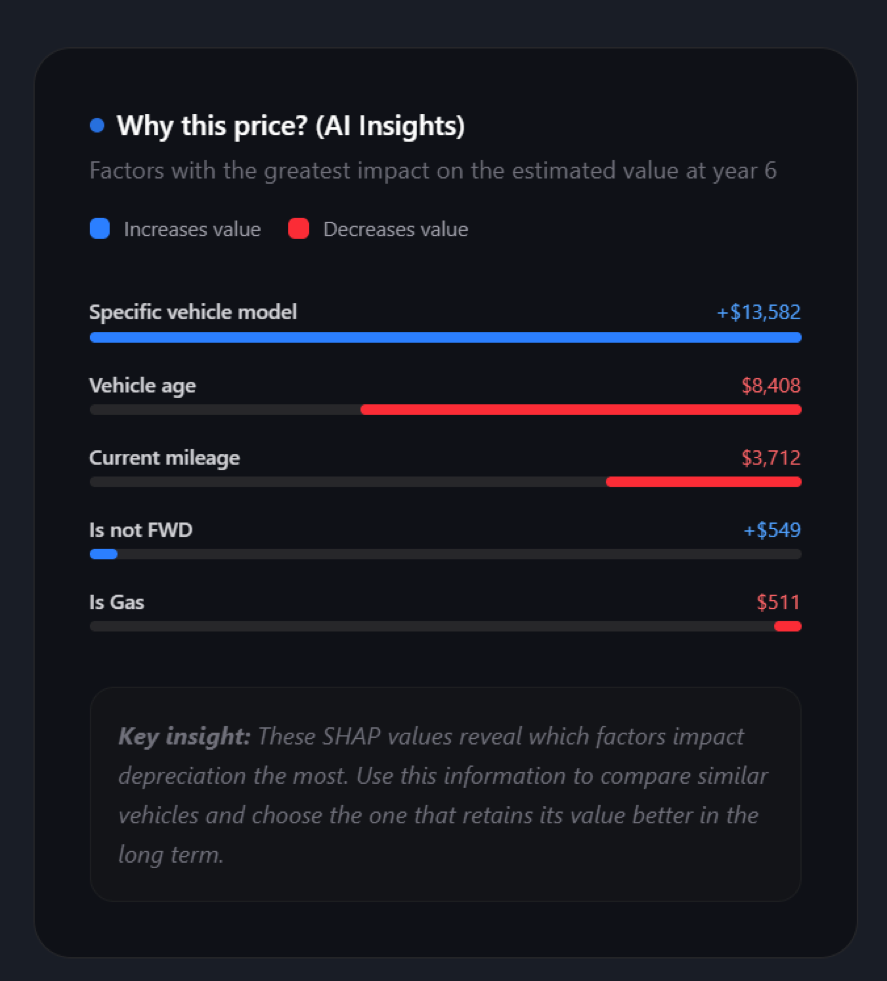
Tree ensembles predict well but are opaque. A SHAP explainer built on the final model decomposes each prediction into a base value (the average prediction) plus the contribution of each feature, so the interface can show the five factors that most raise or lower a specific vehicle’s value at year six.

Across the test set of almost 36,000 vehicles, the vehicle’s age is by far the most influential feature, which is what traditional calculators rely on. Mileage, engine power and the specific model follow, and together the remaining features move the value substantially beyond what age alone explains.

Interface

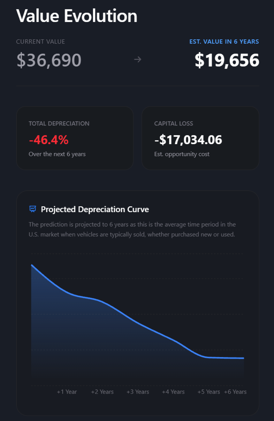
The interface is a single page. A form adapts to new or used vehicles and uses controlled inputs for low-cardinality fields, so requests match the categories the model knows. Results appear as a six-year value curve with the factors behind the prediction.

Out-of-time validation

The model was trained on 2021 data. To test it against the future it was trying to predict, about 2,300 real listings from January 2026 were collected through the MarketCheck API and stored in SQLite, then predicted with the 2021 model as if it had travelled five years forward.

Out-of-time metric (2,293 predictions)	Value
MAE	$4,853
RMSE	$17,448
MAPE	19.5%
Predictions within 15% of the real price	49.5%

Half the predictions landed within 15% of the real price. Error concentrated in brands with short sales histories or luxury segments: Porsche had the highest MAE ($33,373) and Tesla the lowest hit rate (6.8%), while GMC exceeded 70%. The 2021–2026 period included cumulative inflation, the semiconductor shortage and shifts in demand, none of which a model trained on 2021 prices can see. The results suggest the model captures relative depreciation better than nominal future prices, which would need macroeconomic adjustment.

Process

Development combined CRISP-DM for the data work with iterative delivery for the software, integrating every component from the first iteration:

1. A deployed backend serving a mock model behind a provisional API contract, and an unstyled form consuming it.
2. The first trained model, selected by cross-validation, behind the same contract, so the frontend needed no changes.
3. The tuned model with SHAP explanations added to the endpoint, and a redesigned interface.

Limitations and future work

• Data. Training data ends in 2021 and covers the U.S. market. Ferrari and Aston Martin were removed for having too few, too extreme listings, some of them collector vehicles that appreciate.
• Long-horizon uncertainty. Macroeconomic factors dominate five-year error. Adding economic variables, continuous retraining or transfer learning would address this.
• Market. The approach transfers to other markets, including Spain, given a comparable dataset, for example through collaboration with second-hand sales platforms.